ベクトル解析の公式の一覧(ベクトルかいせきのこうしきのいちらん)では、3次元空間におけるベクトル解析の公式の一覧を与える。
内積と外積
ここで , , は任意のベクトルである。また重複添え字については和を取る(アインシュタインの縮約記法)。 はレヴィ=チヴィタ記号、 は , がなす角である。
内積
外積
スカラー三重積
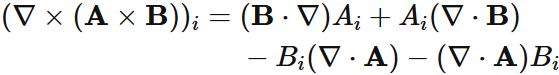
ベクトル三重積
ヤコビ恒等式
四重積
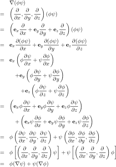
微分公式
ここで , は任意のベクトル場, は任意のスカラー場である。
ヘルムホルツ分解
積分公式
ここで , , は任意のベクトル場, , は任意のスカラー場である。また, は空間領域, はその境界, は面, はその法線ベクトル ( の場合 は外向きに取る), は面要素ベクトルである。閉曲線 に関する線積分 は法線 に対応する向きとする。
ガウスの発散定理および関連する公式(最後の等式はグリーンの定理である)
ストークスの定理および関連する公式
曲線座標
曲線座標における勾配、発散、回転、ラプラシアン、物質微分の公式。
円柱座標
円柱座標 と直交座標 の変換
単位基底ベクトル
計量
体積要素
勾配
発散
回転
ラプラシアン (スカラー場)
ラプラシアン (ベクトル場)
物質微分
球座標
球座標 と直交座標 の変換
単位基底ベクトル
計量
体積要素
勾配
発散
回転
ラプラシアン (スカラー場)
ラプラシアン (ベクトル場)
物質微分
直交曲線座標
3次元ユークリッド空間 の曲線座標 について、その座標系で計量が
という対角形になるとき、これを直交曲線座標と呼ぶ。この座標系に付随する規格化された基底ベクトルを とする。
体積要素
勾配
発散
回転
ラプラシアン (スカラー場)
物質微分
脚注